All-pairs Centrality: Mapping Landscape Connectivity
Three centrality metrics, which consider connections between all pairs of sites (nodes) on a landscape, are analogous to the linkage mapping methods described above: shortest-path betweenness, current flow betweenness, and min cost flow betweenness (Ahuja et al. 1993; Newman 2005; Freeman et al. 1991).
As described above, shortest-path betweenness centrality identifies the one or several shortest (geodesic) paths that connects each pair of nodes on a graph, and counts the number of such shortest paths in which a node participates (Borgatti & Everett 2006). The loss of a node that lies on a large proportion of the shortest paths in the network would disproportionately lengthen distances or transit times between nodes (Brandes 2001). Like least-cost path, betweenness centrality inherently assume optimal paths and thus global knowledge of landscape by the dispersing individual (Freeman 1977).
Current flow or random-walk betweenness centrality assesses the centrality of a node by how often, summed over all node pairs, the node is traversed by a random walk between two other nodes (Newman 2005). Thus this metric counts essentially all paths between nodes, not just the shortest, and is analogous to the behavior of electrical flow in circuits (McRae et al. 2008).
Approximation of shortest-path and current-flow betweenness centrality
Beginning in version 1.2, the CAT's python-based all-pairs centrality functions (shortest-path BC and current-flow BC) by default use algorithms that approximate the exact solutions (Brandes and Fleischer 2005, Brandes and Pich 2007). The exact algorithms also remain available as described below. When used with the default error tolerance values, these approximations provide solutions that are correlated by >99% with the exact solutions, while requiring between 0.1 and 10% of the computational time needed by the exact solutions. This allows BC metrics to be derived for large graphs that were not previously computationally feasible to analyze.
Network flow centrality
Several centrality metrics based on network flow have been proposed in the field of social network theory (Freeman et al. 1991; Borgatti and Everett 2005). In a max-flow algorithm, each edge is assigned a flow which maximizes total flow between a pair of nodes . Flow betweenness centrality bases the importance of a node on the portion of the maximum flow which must pass through that node, summed over all node pairs (Freeman et al. 1991; Borgatti and Everett 2006). However, in graphs such as the landscape lattices considered here, where all nodes have similar numbers of edges, a large number of equivalent maximum flow paths exist. We have found that the flow betweenness centrality of Freeman et al. (1991) was less informative than a centrality metric based on minimum-cost-maximum-flow (Ahuja et al. 1993). Whereas least-cost path and max-flow algorithms only consider cost and capacity, respectively, min-cost-max-flow algorithms simultaneously consider cost and capacity to identify the set of edges or nodes of minimum cost that permit a set level of flow (Ahuja et al. 1993). The min-cost-max-flow betweenness centrality metric we developed first calculates the max-flow between a pair of nodes, and then maps the min-cost path for that flow. The importance of a node is based on the portion of the min-cost-max-flow which must pass through that node, summed over all node pairs. Simple cost value might assign private lands greater cost of public lands, reflecting common policies that seek to develop options for species conservation on public lands before regulating management of private lands. Or a uniform (positive non-zero) cost value may be used, which results in identification of the maximum flow path of minimum total area.
While pairwise linkage analysis using min-cost-max-flow is relatively rapid (
Exercise 1), the computational time required for min-cost-max-flow betweenness centrality analysis of large graphs is currently on the order of thousands of hours. In some contexts, it may be preferable and more feasible to analyze a ‘bounded-distance’ min-cost-max-flow centrality metric that considers only pairwise relationships of nodes separated by less than a threshold distance. Borgatti and Everett (2006) suggested use of ‘bounded-distance’ betweenness in contexts where very long connections may be expected to be less relevant to system processes.
Given that it is computationally challenging to derive minimum-cost-maximum-flow BC over regional extents, we suggest regional planning efforts compare results from shortest-path and current-flow BC analyses. Shortest-path BC results identify the minimal set of linkages whose loss would greatly reduce regional connectivity. In contrast, the zones identified by current-flow BC assist in incorporating redundancy within a linkage network, which may be important for designing networks that are resilient to changing climate and land-use patterns or environmental catastrophes. Areas of high current flow BC may indicate pinchpoints where much potential dispersal flow encounters relatively constrained linkages. Higher-resolution analysis of individual linkages (
Exercise 2) can be placed in context using the priority assigned to the linkage area in regional analyses.
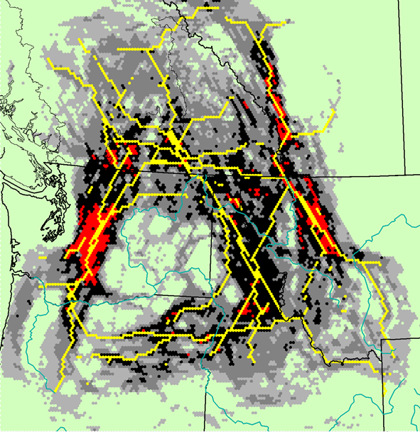
Shortest-path BC results overlaid on current flow BC results for wolf habitat in
the northwestern US and southwestern Canada.