Example 1: Shortest-path betweenness centrality (BC)
Case study: Analysis of landscape permeability in California with all-pairs shortest-path betweenness centrality
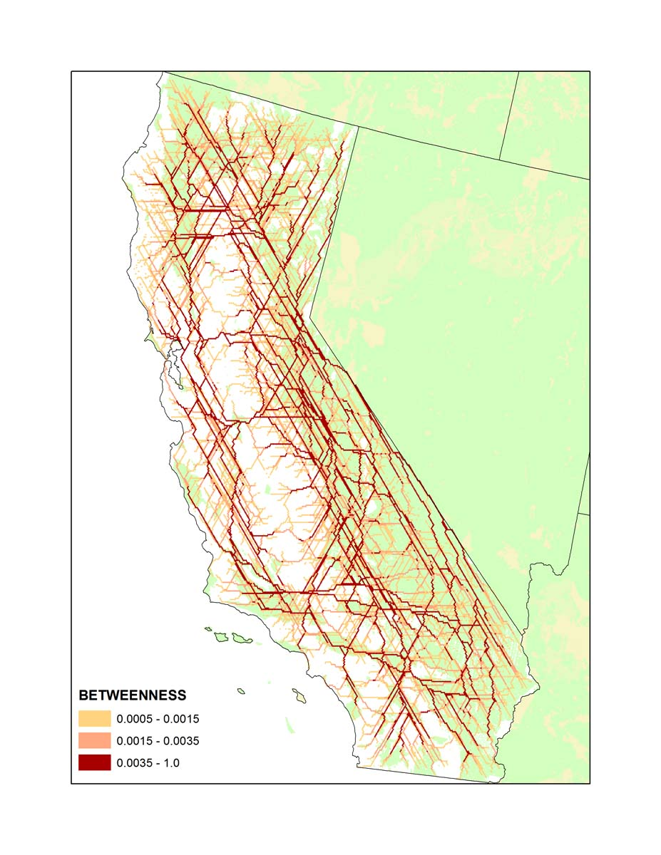
As part of the development of the report "California Essential Habitat Connectivity Project: A Strategy for Conserving a Connected California", Spencer et al. (2010) developed a data layer representing landscape resistance for the state of California. This data is used here to develop an example of how centrality analysis may be applied to such generalized representations of landscape pattern and composition to produce connectivity results that are not species-specific. The resistance data, based on landscape features such as vegetation, roads, and human land use, was on an ordinal scale of 1 to 25. Because the Toolkit expects habitat data to be scaled as conductance (i.e., here worst=1, best=25) rather than resistance, we first inverted the scaling. (In retrospect, it would be technically more correct to have taken the reciprocal of conductance to derive resistance. However, an ordinal scale cannot be assumed to directly represent conductance, so the best approach may be to try several different transformations.) We then squared the values to accentuate the contrast between poor and good values, a step that is often necessary when input data are on an ordinal scale rather than e.g., representing probabilities of occurrence. 82,000 hexagons of 5 square kilometers each were used to represent the region in a graph format. The exact algorithm for shortest-path betweenness centrality analysis required 0.2 GB and 20 hours to complete. Approximate solutions required less than 1 hour. The results are shown here overlaid on a background showing public lands within California. This is an exploratory analysis, so may be most appropriately used as a tool for comparison with results from other methods described in Spencer et al. (2010).