Three Methods for Connectivity Analysis
This software allows users to apply three types of linkage mapping methods: shortest or least-cost path, current flow, and network flow (specifically min-cost-max-flow). These methods consider respectively 1) the single shortest path, 2) probabilistic flow across all possible paths, and 3) optimal flow which considers, but may not use, all possible paths.
3 pairwise linkage mapping methods
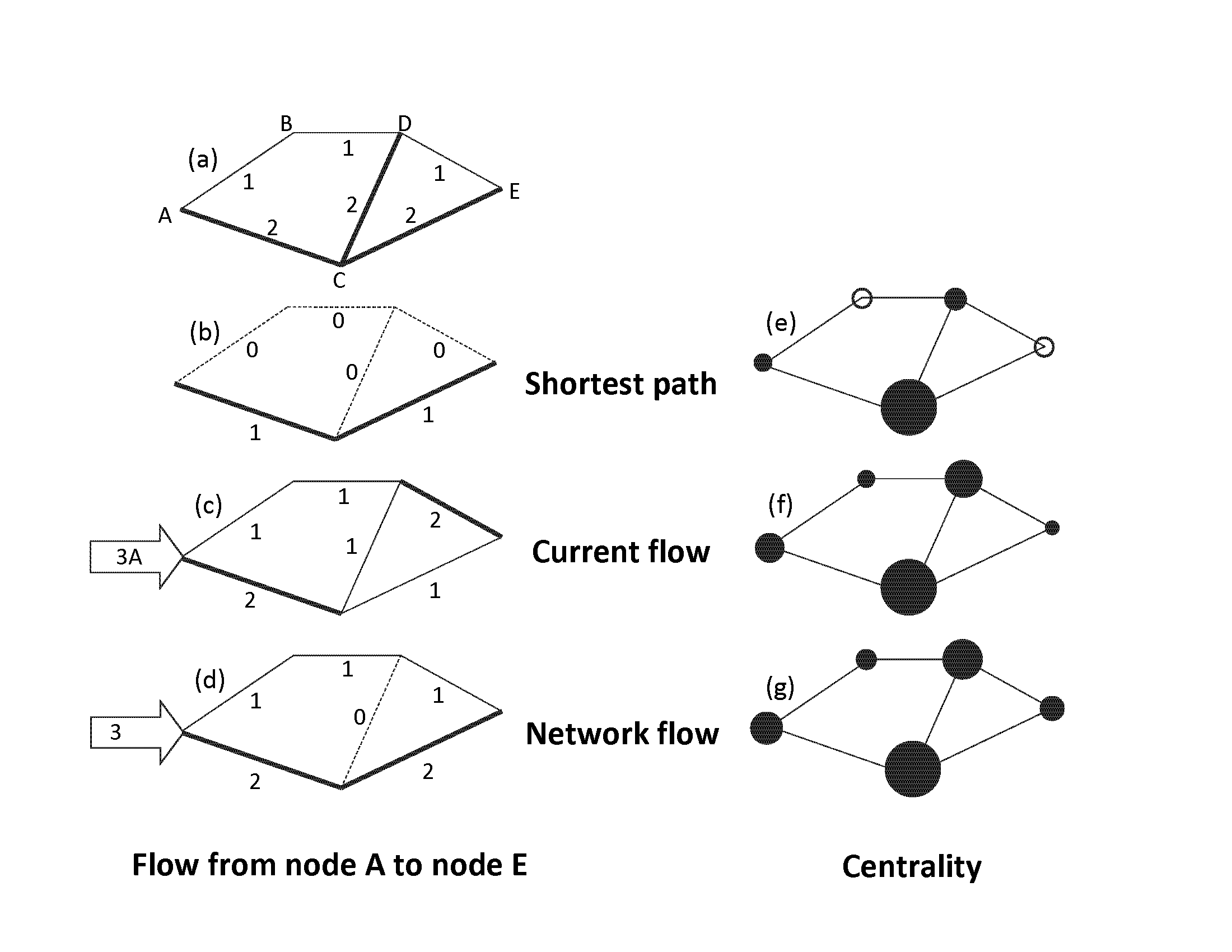
We can illustrate the contrast between these methods with a simple graph with 5 nodes and 6 edges (below). a) Edge values shown here may be derived from habitat suitability models, and may be represented as proportional to conductance (circuit flow) and flow capacity (network flow), and inversely proportional to cost (not shown); b) A shortest- or least-cost path solution assigns all priority to the path A-C-E; c) current flow analysis with a 3 ampere source at A identifies edges A-C and D-E as showing highest current flow, with all other edges showing lower but non-zero current levels; d) Network flow maximum-flow analysis identifies both a high-capacity path A-C-E and a lower capacity path A-B-D-E, but none of the maximum flow will transit edge C-D. If all edges had the same cost, the min-cost-max-flow solution from A to E would be identical to the max-flow solution on this simple graph.
3 analogous centrality metrics
The 3 centrality metrics considered here are variants of betweenness centrality (BC), in that they measure to what extent a node contributes to paths or flows between all other nodes (Borgatti & Everett 2006; Newman 2010). Shortest-path BC identifies the one or several shortest (geodesic) paths that connect each pair of nodes on a graph and counts the number of such shortest paths in which a node is included (Borgatti & Everett 2006). Current-flow BC assesses the centrality of a node on the basis of how often, summed over all node pairs, the node is traversed by a random walk between 2 other nodes (Newman 2005). Minimum-cost-maximum-flow BC evaluates a node’s contribution to connectivity on the basis of portion of the minimum-cost-maximum-flow that must pass through that node, summed over all node pairs (Freeman et al. 1991). In the figure below, shortest-path BC (e) resembles shortest-path results between a node pair (b) because it assigns high centrality to node C, which lies on the shortest path between many node pairs, and zero centrality to nodes (B, E), which do not lie on the shortest paths between any pair of nodes. Current-flow BC (f) ranks the importance (for facilitating flow) of nodes similarly as does shortest-path BC, but centrality values are more evenly distributed among nodes and there are no nodes of zero centrality due to the model’s random-walk behavior. Maximum-flow BC ranks nodes similarly to current flow BC, but values are distributed more evenly (g). If all edges have equal cost, results of minimum-cost maximum- flow BC (not shown) resemble maximum-flow BC.
Graphs are classified as either directed or undirected dependent on whether the edge weight (data representing attributes such as cost, conductance, or capacity) of edge i-j (from node i to j) equals the weight of the edge j-i. All the metrics described here, with the exception of those based on time series analysis, can use undirected graphs with edge weights derived from the mean weight of the two end nodes connecting that pair. Untransformed habitat values from a habitat model may be used as weights for current flow and network flow algorithms. The reciprocal of habitat value is typically used to represent cost in calculating the least-cost or betweenness metrics, although other transformations are possible as well.
Figure adapted from Carroll et al. 2011