Exercise 4 - Mapping connectivity under climate change: analysis of time series
In addition to allowing generation of graphs from single data layers, the Connectivity Analysis Toolkit also allows creation of graphs from a series of related layers of identical dimensions. These are typically 'time series' depicting e.g., how a landscape's suitability for a species is projected to change over time (with climate change, forest succession, or restoration).
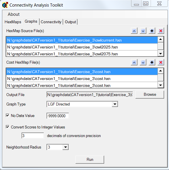
1) Graphs Tab –
We will use 6 hxn files that have previously been created to create the LGF (LEMON graph format) input file we will use in the climate connectivity analysis. These files contain data depicting habitat suitability for Northern Spotted Owl in the years 1961-1990 (“current”), 2011-2040 ("2025"), and 2061-2090 ("2075").
As this capability is not present in your version of the CAT (version 1.0), please follow along as the example is demonstrated on the screen.
Press the + tab above the upper box and add the file owlcurrent.hxn to the upper box (Hexmap Source File).
Press the + tab above the upper box and add the file owl2025.hxn to the upper box. It will be listed below the spowcur.hxn file.
Press the + tab above the upper box and add the file owl2075.hxn to the upper box.
Three hxn files are now listed in the upper box.
Press the + tab above the lower box and add the file cost.hxn to the lower box (Cost Hexmap).
In this example, we have no data on how cost varies over time, so we use the same (area-based or uniform) cost hxn for all timesteps.
Do this a second and third time until 3 hxn files are listed in the lower box.
Set graph type as LGF Directed.
Set the Output file name as owl3n.lgf
Leave checked ‘No Data Value -9999’.
Set the decimals of ‘convert scores to integer values’ as 3.
Set Neighborhood Radius to 3.
Press Run.
Examine the file owl3n.lgf in a text editor. Note how the node and arc sections of this file are created and attributed.
Examine the file owl3n.tab in a text editor. This file specifies the correspondence between nodes in the time-series graph and hexagons in the input hxn files.
3) Connectivity Tab -
Browse and locate the graph file, owl3n.lgf.
In the Connectivity Tab, set the Function as ‘Time-Series Minimum Cost Flow’.
Browse and name the output file: owl3nout. [NOTE: Do not add a file suffix (e.g., .tab), or networkflow.exe will crash).
Press Run to run the analysis.
The progress of the analysis will be displayed in the ‘Output’ tab.
4) Working with the CAT timeseries output files
The CAT will produce a separate output file for each 'layer' in the time-series graph. Thus a graph created from 3 hxn files will result in 3 * 2 = 6 output files. Numbering of the output files is done starting with '0', so the output from the first step of the first time step will be named owl3nout_0_0.tab. These files contains the hex_id and outgoing flow values for each layer. These files can be joined to the shapefile output in ArcGIS as described in Exercise 1. The output files from the first layer in the second through final time steps will be most relevant to planning.